PID Loops - How to Control Your Projects!

2023-10-27 | By Antonio Velasco

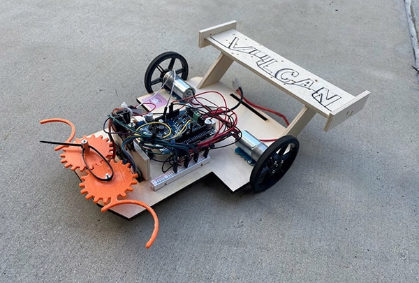
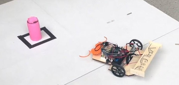
“Make a rover that tracks and follows a pink can!” Seems like a pretty straightforward task, right? My team was given this task in our Freshman Introduction to Engineering course, then armed with a PixyCam, an Arduino, and two good motors. We felt confident we’d be able to knock this one out of the park within the two-hour lab period.

We set up the rover to turn left or right depending on where the can is in the range of the frame and to move straight when the can is in the center. It felt like a simple and clean solution to the problem, and with high hopes, we went to test the rover. It didn’t work out as we had hoped.

PID Loops - How to Control Your Projects

When we flipped the rover on, it would “jitter” back and forth (rapidly turning left and right) like it was freaking out whenever the can was in its sight. We thought it could be a motor or a software issue, but when other teams started to have the same issue, we realized that there had to be something more than an incorrect line of code–there was a missing piece to the puzzle that they had intended us to find on our own.

There simply was no control over the rover. At first, we figured that the turn speed was too strong and that when it would try to turn left or right to adjust itself, the rover would move too much in one direction, and the code would make it correct itself by forcing itself to turn again. This proved to be true as we tried to make the detection parameters more forgiving and the turns slower by turning down the motor speed, but while it solved the jittering, this ended up making the rover much slower and less responsive when we’d move the can. Then, I thought, why not adjust the turn speed based on the position of the can? It’d allow the robot to turn only as much as it needed and would result in a happy medium rather than plugging and chugging values until it worked.

Such was my introduction to what I’ve come to know as PID Control.

What is PID?

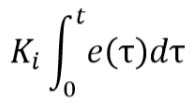
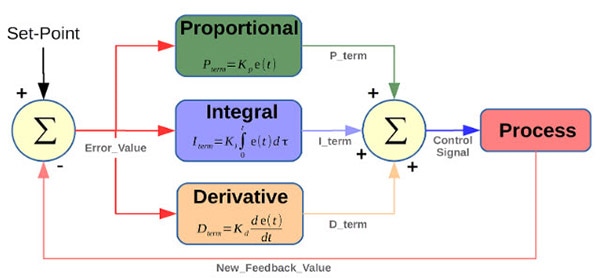
PID stands for Proportional, Integral, and Derivative–all pieces to a puzzle that make movement smoother. PID control is used everywhere, from pneumatics to your car’s cruise control. It all boils down to a control system represented by this equation:

PID Loops - How to Control Your Projects

Looks pretty daunting though, right? Let’s break it down.

P- Proportional

The P stands for proportional, meaning that the output value would be adjusted proportionally to what it would need to be. In our case, it’s the turn speed. If the object was further to the left or right, the turn speed would be adjusted depending on how far it is. Conversely, if the object was closer, the turn speed would be lessened as to not oversteer. This can be displayed in an equation where we have a constant that is affected by the position of the pink can in the camera. While this does help the rover get back on track, the turn speed can be further tuned by looking at its rate of change.

PID Loops - How to Control Your Projects

Where Kp is the constant and e(t) is an equation that determines the difference/relative distance.

D-Derivative

The D stands for derivative, meaning that the output value would be adjusted as to not have too sharp of a turn even when the can seems to be far away. We’ll skip “I” for now as D would be a better next step. While our turn speed is tuned to be adjusted based on the pink can’s relative location, we don’t want to incur very sharp turns as it may result in the rover going off-course or turning too much, missing the center line we want it to end up at. Derivative control helps to mitigate that by implementing a control for the rate of change, or in our case, the rate at which the turn speed would change. Like when a driver turns a steering wheel, they slowly ease into an angle over time as opposed to sharply turning–that’d make cars way harder to control. For example, if the can is very far to the left, we’d have derivative control to prevent the turn speed from hitting a very high value, which would jerk the rover or possibly misplace it. This can be displayed in an equation where we have a constant that is affected by the derivative, or rate of change, of our turn speed.

PID Loops - How to Control Your Projects

Where Kd is a constant and e(t) is an equation that determines the difference/relative distance, with a derivative with respect to time attached to it to determine the rate of change. This can be represented in code by having a variable that is calculated by finding the difference between the initial and current position every loop.

I-Integral

Finally, we have I, which stands for integral, allowing us to measure our relative change over time. This is great for fine-tuning as it would allow the rover to correct itself after a certain amount of time given that it is off course. Say that, for some reason, our rover is slightly off the center track, but not enough for the proportional turn speed to increase enough to get it back on track at a reasonable time. The derivative control wouldn’t be helpful in this case, so we turn to integral control to get us back on track. Over time, it would measure how far the rover is from the central track line and eventually, it would add up the margin of error and correct itself. For example, if the can is very slightly to the right, and the proportional control uses a very small value to turn because of how close it is, the integral control would measure this error over a period of time and eventually hit a value that would correct itself. This is displayed in an equation with a constant that is affected by an integral, which would slowly rise if the error were constant.

PID Loops - How to Control Your Projects

Where Ki is a constant and e(t) is an equation that measures the distance between our current trajectory and the intended trajectory, which is then integrated with respect to time. This can be represented in code by having a variable that is increased by a certain amount with every loop.

The Pieces Coming Together

We ended up getting the rover working with a combination of the three–using proportional control to increase the turn speed if the can is further to the side, using derivative control to prevent jerking and to control the turn speed, and finally using integral control at very close values. This was implemented through coding in variables that were affected by the PID equation, incorporating allparts of it. In a lot of cases, you will have to tune the constants for each part of the equation to allow an optimum control system.

PID Loops - How to Control Your Projects

Each part of the equation allows the system to perform tasks with a power that is not too strong, not too weak, but just right. This can be applied to a myriad of projects, whether you’re creating a rover like me or a robot arm that picks up items. Whatever it is that you do, make sure you control yourself!