Build a Machine Learning Application with a Raspberry Pi

Developers looking to evaluate machine learning methods find a growing array of specialized hardware and development platforms that are often tuned to specific classes of machine learning architecture and application. Although these specialized platforms are essential for many machine learning applications, few developers new to machine learning are ready to make informed decisions about selecting the ideal platform.

Developers need a more accessible platform for gaining experience in development of machine learning applications and a deeper understanding of resource requirements and resulting capabilities.

As described in the DigiKey article “Get Started with Machine Learning Using Readily Available Hardware and Software”, development of any model for supervised machine learning comprises three key steps:

• Preparation of data for training a model
• Model implementation
• Model training

Data preparation combines familiar data acquisition methods with an additional step required to label specific instances of data for use in the training process. For the final two steps, machine learning model specialists, until recently, needed to use relatively low-level math libraries to implement the detailed calculations involved in model algorithms. The availability of machine learning frameworks has dramatically eased the complexity of model implementation and training.

Today, any developer familiar with Python or other supported languages can use these frameworks to rapidly develop machine learning models able to run on a wide array of platforms. This article will describe the machine learning stack and training process before getting into how to develop a machine learning application on a Raspberry Pi 3.

Machine learning stack

To support model development, machine learning frameworks provide a full stack of resources (Figure 1). At the top of a typical stack, training and inference libraries provide services for defining, training, and running models. These models in turn build on optimized implementations of kernel functions such as convolutions and activation functions such as ReLU, as well as matrix multiplication and others. Those optimized math functions work with lower level drivers that provide an abstraction layer to interface with a general purpose CPU, or take full advantage of specialized hardware such as a graphics processing unit (GPU) when available.

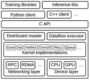
Figure 1: In the typical machine learning stack, higher level libraries provide functions to implement neural networks and other machine learning algorithms, drawing on specialized math libraries that implement kernel functions optimized for CPUs and GPUs in the underlying hardware layer. (Image source: Google)

With the availability of machine learning frameworks such as TensorFlow that provide these stacks, the development process for implementing machine learning in an application has become largely the same regardless of hardware targets. The ability to leverage TensorFlow across different hardware platforms allows developers to begin exploring model development on relatively modest hardware platforms, and then leverage that experience in developing machine learning applications on more robust hardware.

It’s expected that specialized high performance artificial intelligence (AI) chips will eventually provide developers the ability to implement sophisticated machine learning algorithms. Until then, developers can begin to evaluate machine learning and create real machine learning applications using general purpose platforms, including the Raspberry Pi Foundation’s Raspberry Pi 3, or any of the readily available development boards based on general purpose processors such as Arm^® Cortex^®-A series MCUs or Arm Cortex-M series MCUs.

The Raspberry Pi 3 offers some immediate advantages as a development platform for machine learning applications. Its Arm Cortex-A53 quad core processor provides significant performance capabilities, and the core’s NEON single instruction, multiple data (SIMD) extensions are capable of performing a certain level of multimedia and machine learning type processing. However, developers can easily extend the base Raspberry Pi 3 hardware platform with any number of available compatible hardware add-ons.

For example, to create the kind of machine learning image recognition system described below, developers can add a camera such as the 8 megapixel Raspberry Pi Camera Module v2 or its low-light Pi NoIR camera (Figure 2).

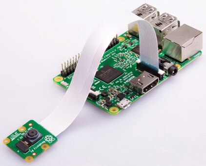
Figure 2: Low-cost boards such as the Raspberry Pi 3 provide a useful platform for machine learning development, supporting add-ons such as camera modules for developing image classification applications. (Image source: Raspberry Pi Foundation)

On the software side, the Raspberry Pi community has created an equally rich ecosystem in which developers can find distributions including complete pre-compiled binary wheel files for installing TensorFlow on a Raspberry Pi. TensorFlow provides these wheel files for Python 3.4 and 3.5 on the Raspberry Pi wheels repository piwheels.org. Alternatively, because Docker now officially supports the Arm architecture, developers can use suitable containers from dockerhub.com.

Implementing a machine learning model

Using this combination of software, a Raspberry Pi 3, and a camera module, developers can build a simple machine learning gesture recognition application using sample code from Arm. This application is designed simply to detect when the user has made a specific gesture: in this case, throwing hands up in the air in a sort of celebratory gesture.

To start, use a Python script (record.py) to record short video clips of someone performing the same gesture a few times. Because this application is meant to be as simple as possible, the next step begins training using the Keras machine learning application programming interface (API) embedded in TensorFlow. In this example, the training process is defined in another Python script (train.py) that includes the Keras model definition and training sequence (Listing 1).

Copy
def main():
    .
    .
    .
    model_file = argv[1]
    recording_files = argv[2:]
    feature_extractor = PiNet()
    .
    .
    .
    for i, filename in enumerate(recording_files):
        stdout.write(' %s' % filename)
        stdout.flush()
        with open(filename, 'rb') as f:
            x = load(f)
            features = [feature_extractor.features(f) for f in x]
            label = np.zeros((len(recording_files),))
            label[i] = 1.          # Make a label with a 1 in the column for the file for this frame
            xs += features         # Add the features for the frames loaded from this file
            ys += [label] * len(x) # Add a label for each frame in the file
            class_count[i] = len(x)

    print("Creating a network to classify %s" % ', '.join(recording_files))
    classifier = make_classifier(xs[0].shape, len(recording_files))

    print("Training the network to map high-level features to %d categories" % len(recording_files))
    classifier.fit([np.array(xs)], [np.array(ys)], epochs=20, shuffle=True)

    print("Now we save this model so we can deploy it whenever we want")
    classifier.save(model_file)


def make_classifier(input_shape, num_classes):
    """ Make a very simple classifier
        Layers:
            GaussianNoise: Add random noise to prevent our classifier memorizing specific examples.
            Flatten: The input may come from a layer with shape (x, y, depth); flatten it to 1D.
            Dense: Provide one output per class scaled to sum to 1 (softmax) """

    # Define a simple neural network
    net_input = keras.layers.Input(input_shape)

    noise = keras.layers.GaussianNoise(0.3)(net_input)
    flat = keras.layers.Flatten()(noise)
    net_output = keras.layers.Dense(num_classes, activation='softmax')(flat)

    net = keras.models.Model([net_input], [net_output])

    # Compile a model before use. The loss should match the output activation function, e.g.
    # binary_crossentropy for sigmoid, categorical_crossentropy for softmax, mse for linear.
    # Adam is a solid default optimizer, we can leave the learning rate at the default.
    net.compile(optimizer=keras.optimizers.Adam(),
                loss='categorical_crossentropy',
                metrics=['accuracy'])
    return net

Listing 1: In this snippet from the Arm sample application repository, the training process combines a pre-trained model with the simple classifier required for this application. (Code source: Arm)

Despite the apparent simplicity of this model, it is actually quite sophisticated, using a technique called transfer learning. Transfer learning uses a proven model trained with one data set as the starting point for training a model targeting a different but related problem set. In this case, this application uses an optimized convolutional neural network (CNN) model from Google's MobileNet model set.

Developed by Google, MobileNet models are CNNs trained on a subset of the de facto standard ImageNet dataset of labeled images. The distinguishing characteristic of MobileNet models is that they are configured to support the kind of reduced resource requirements needed for mobile devices or general-purpose boards such as the Raspberry Pi. The cost of this resource reduction is reduced accuracy. Although these models provide a level of accuracy that will fall well below requirements for mission critical applications, MobileNet models can prove useful for more relaxed requirements and for serving as the base model in transfer learning.

For this application, the train.py script creates a feature extractor using a MobileNet model where the final classification layer has been removed:

feature_extractor = PiNet()

The PiNet function simply reads the modified MobileNet model included in the code repository.

The application then uses that modified model to create the feature set (features) for this training data set of images:

features = [feature_extractor.features(f) for f in x]

where x is an array containing frames produced by record.py during the initial data collection step.

Finally, the train.py script uses the Keras fit method to train the model and the save method to save the final model for use during inference:

classifier.fit([np.array(xs)], [np.array(ys)], epochs=20, shuffle=True)

classifier.save(model_file)

To use the resulting model file for inference, invoke another script, run.py. The key design pattern in this script is the endless loop, which takes each frame, calculates features (extractor.features), uses the same classifier for inference (classifier.predict), and generates the predictions for the label (np.argmax). The predictions are simply whether the target gesture has occurred, or not (Listing 2).

Copy
    while True:
        raw_frame = camera.next_frame()

        # Use MobileNet to get the features for this frame
        z = extractor.features(raw_frame)

        # With these features we can predict a 'normal' / 'yeah' class (0 or 1)
        # Keras expects an array of inputs and produces an array of outputs
        classes = classifier.predict(np.array([z]))[0]

        # smooth the outputs - this adds latency but reduces interruptions
        smoothed = smoothed * SMOOTH_FACTOR + classes * (1.0 - SMOOTH_FACTOR)
        selected = np.argmax(smoothed) # The selected class is the one with highest probability

        # Show the class probabilities and selected class
        summary = 'Class %d [%s]' % (selected, ' '.join('%02.0f%%' % (99 * p) for p in smoothed))
        stderr.write('\r' + summary)

Listing 2: This snippet from the Arm sample run.py script demonstrates the basic design pattern for inference, using the same pretrained model to extract features and the same classifier to perform inference. (Code source: Arm)

Multi-classification models

Developing an application to detect one class of input such as a single gesture is a worthwhile exercise in machine learning development, but machine learning applications are typically intended for multi-class classification. Another Arm sample application demonstrates the steps needed to do just that, and provides a more complete example of the steps typically required to complete multi-classification model development. For example, the single gesture application requires no significant data preparation other than capturing the desired gesture. In contrast, the multi-classification application involves substantial data capture and an associated development step to label the captured video with the target class (the gesture) using a Python script that Arm provides. In this case, the developer captures short video clips of different actions such as entering or leaving a room, pointing at a light (to turn it on or off), and making different gestures to start or stop music playing. Using the classify.py script, view the images and enter the appropriate label (an integer corresponding to each action). After labeling is complete, hold back about 10% of the labeled data for use to test the model as discussed below.

With the training data and reserved test set in hand, the next step involves creation of the model itself. Unlike the heavy use of a pretrained model in the single gesture application, this application builds a complete CNN model. In this case, use a series of Keras statements that build a model layer by layer using Keras functions that build a 2D convolution layer (Conv2D), add an activation layer (Activation), a pooling layer (MaxPooling2D), and so on (Listing 3).

Copy
def main():
    if len(argv) != 3 or argv[1] == '--help':
        print("""Usage: train.py TRAIN_DIR VAL_DIR...
Save TRAIN_DIR/model.h5 after training a conv net to distinguish between images in its subdirs.""")
        exit(1)

    train_data_dir = argv[1]
    val_data_dir = argv[2]
    nb_train_samples = len(glob('%s/*/*.png' % train_data_dir))
    nb_classes = len(glob('%s/*/' % train_data_dir))
    batch_size = 100

    model = Sequential()
    model.add(Conv2D(32, (3, 3), input_shape=(128, 128, 3)))
    model.add(Activation('elu'))
    model.add(MaxPooling2D(pool_size=(2, 2)))

    model.add(Conv2D(32, (3, 3)))
    model.add(Activation('elu'))
    model.add(MaxPooling2D(pool_size=(2, 2)))

    model.add(Conv2D(64, (3, 3)))
    model.add(Activation('elu'))
    model.add(MaxPooling2D(pool_size=(2, 2)))

    model.add(Flatten())
    model.add(Dense(64))
    model.add(Activation('elu'))
    model.add(Dropout(0.5))
    model.add(Dense(nb_classes))
    model.add(Activation('softmax'))

    model.compile(loss='categorical_crossentropy',
                  optimizer='adam',
                  metrics=['accuracy'])

Listing 3: The Arm multi-classification sample application illustrates the use of Keras functions to build a convolutional neural network layer by layer. (Code source: Arm)

This model also introduces the concept of a dropout layer (Dropout in Listing 3), which provides a form of model optimization called regularization. In model training algorithms, a regularization factor reduces the model's tendency to chase every feature, which can cause overfitting in models. Dropout performs this same function by literally dropping a random set of neurons out of the processing chain (Figure 3).

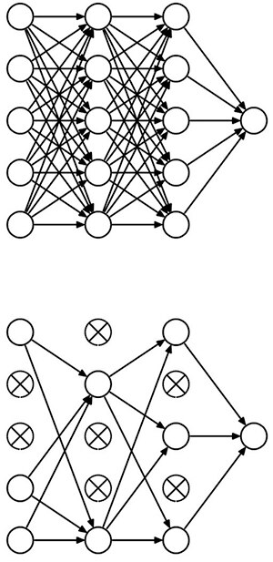
Figure 3: Dropout provides regularization in a deep neural network by randomly disabling neurons, effectively converting a fully connected neural network (top) to a less dense version (bottom). (Image source: University of Toronto)

With the completed model in hand, use conventional training methods built into TensorFlow and other frameworks. The actual training process can take hours, days, even weeks for very complex models. Although developers typically use GPUs to speed training, the use of transfer learning, as in the earlier application, can help reduce training times. However, the use of a complete model in this multi-classification application translates into significantly greater training times. Arm notes that training time for this application could be significant on a Raspberry Pi. Instead, Arm suggests developers install TensorFlow on their own workstation, perform training on the workstation, and copy the trained model back to the Raspberry Pi.

When using the model, the inference process largely follows the same series of calls shown earlier for the single gesture application. For this application, of course, the inference process uses the custom model described in Listing 3, rather than the single gesture pre-trained model and shallow classifier described in Listing 1. Beyond that obvious difference, multi-classification model development adds an additional step for testing the model before production use.

In this test phase, run the model just as for production inference, but instead of using some new input data, use the 10% labeled data held back from training. Because the correct answer for inference of each test image is already known, a test script can record the actual accuracy results for comparison with the accuracy results achieved at the completion of training.

Beyond its basic benefits as a hard metric, the test phase and the way the model responds to test data can offer hints on what steps may need to be taken to improve the model. Because this test data comprises the same type of data used in training, a trained model should generate predictions with the same level of accuracy achieved during training itself. For models that exhibit overfitting, reduce the number of input features and apply more robust regularization methods. For models with underfitting, do the opposite; add more features and reduce the amount of regularization.

MCU-based applications

TensorFlow and other frameworks each provide a consistent model development approach that can be applied across a wide range of target hardware platforms. Yet, they are by no means the only approach. When developing machine learning applications on Arm-based platforms, developers can turn to the company's own libraries.

Developed to support Arm Cortex-A series MCUs, the Arm Compute Library provides a full set of functions for implementing CNNs and other machine learning algorithms. For Arm Cortex-M series MCUs, the Arm Cortex Microcontroller Software Interface Standard (CMSIS) includes a neural network (NN) library. Just as CMSIS-DSP extends CMSIS for DSP applications, CMSIS-NN provides machine learning functions for implementing popular NN architectures on Arm Cortex-M-based platforms. For example, use the CMSIS-NN library to implement CNNs on the STMicroelectronics NUCLEO-F746ZG development board, which is built around the STMicroelectronics Arm Cortex-M7-based STM32F746ZG MCU.

To implement a neural network with CMSIS-NN, developers can import an existing model from TensorFlow or other frameworks. Alternatively, they can implement a CNN natively through a series of CMSIS-NN function calls. For example, to implement a CNN able to process the industry standard CIFAR-10 labeled image dataset, the developer would build the model layer by layer, similar to the method shown earlier for Keras. In this case, the CNN layers are implemented as a series of CMSIS-NN function calls. The final softmax layer produces the 10 output neurons required for CIFAR-10 (Listing 4).

Copy
int main()
{
  .
  .
  .
  // conv1 img_buffer2 -> img_buffer1
  arm_convolve_HWC_q7_RGB(img_buffer2, CONV1_IM_DIM, CONV1_IM_CH, conv1_wt, CONV1_OUT_CH, CONV1_KER_DIM, CONV1_PADDING,
                          CONV1_STRIDE, conv1_bias, CONV1_BIAS_LSHIFT, CONV1_OUT_RSHIFT, img_buffer1, CONV1_OUT_DIM,
                          (q15_t *) col_buffer, NULL);

  arm_relu_q7(img_buffer1, CONV1_OUT_DIM * CONV1_OUT_DIM * CONV1_OUT_CH);

  // pool1 img_buffer1 -> img_buffer2
  arm_maxpool_q7_HWC(img_buffer1, CONV1_OUT_DIM, CONV1_OUT_CH, POOL1_KER_DIM,
                     POOL1_PADDING, POOL1_STRIDE, POOL1_OUT_DIM, NULL, img_buffer2);

  // conv2 img_buffer2 -> img_buffer1
  arm_convolve_HWC_q7_fast(img_buffer2, CONV2_IM_DIM, CONV2_IM_CH, conv2_wt, CONV2_OUT_CH, CONV2_KER_DIM,
                           CONV2_PADDING, CONV2_STRIDE, conv2_bias, CONV2_BIAS_LSHIFT, CONV2_OUT_RSHIFT, img_buffer1,
                           CONV2_OUT_DIM, (q15_t *) col_buffer, NULL);

  arm_relu_q7(img_buffer1, CONV2_OUT_DIM * CONV2_OUT_DIM * CONV2_OUT_CH);

  // pool2 img_buffer1 -> img_buffer2
  arm_maxpool_q7_HWC(img_buffer1, CONV2_OUT_DIM, CONV2_OUT_CH, POOL2_KER_DIM,
                     POOL2_PADDING, POOL2_STRIDE, POOL2_OUT_DIM, col_buffer, img_buffer2);

// conv3 img_buffer2 -> img_buffer1
  arm_convolve_HWC_q7_fast(img_buffer2, CONV3_IM_DIM, CONV3_IM_CH, conv3_wt, CONV3_OUT_CH, CONV3_KER_DIM,
                           CONV3_PADDING, CONV3_STRIDE, conv3_bias, CONV3_BIAS_LSHIFT, CONV3_OUT_RSHIFT, img_buffer1,
                           CONV3_OUT_DIM, (q15_t *) col_buffer, NULL);

  arm_relu_q7(img_buffer1, CONV3_OUT_DIM * CONV3_OUT_DIM * CONV3_OUT_CH);

  // pool3 img_buffer-> img_buffer2
  arm_maxpool_q7_HWC(img_buffer1, CONV3_OUT_DIM, CONV3_OUT_CH, POOL3_KER_DIM,
                     POOL3_PADDING, POOL3_STRIDE, POOL3_OUT_DIM, col_buffer, img_buffer2);

  arm_fully_connected_q7_opt(img_buffer2, ip1_wt, IP1_DIM, IP1_OUT, IP1_BIAS_LSHIFT, IP1_OUT_RSHIFT, ip1_bias,
                             output_data, (q15_t *) img_buffer1);

  arm_softmax_q7(output_data, 10, output_data);

  for (int i = 0; i < 10; i++)
  {
      printf("%d: %d\n", i, output_data[i]);
  }

  return 0;
}

Listing 4: In this snippet from the Arm sample CIFAR-10 application, the main routine illustrates the series of calls used to build a CIFAR10 targeted convolutional neural network using the Arm Cortex Microcontroller Software Interface Standard (CMSIS) neural network (NN) library. (Code source: Arm)

General purpose platforms lack the resources to deliver the kind of inference performance possible with GPU-based systems. As a result, these platforms typically cannot reliably support any kind of "real-time" inference of video that is operating at the usual frame rates needed to maintain flicker-free appearance. Even so, the CMSIS-NN CIFAR-10 model described above can achieve inference rates of about 10 per second, which could be fast enough to support relatively simple applications that require limited update rates.

The continued development of reduced models, such as MobileNet and frameworks such as TensorFlow Lite and Facebook's Caffe2Go, offer further options for implementing machine learning on resource-constrained devices for the IoT and other connected applications.

Conclusion

Machine learning applications follow a typical development pattern of data preparation and training that remains conceptually consistent across different target platforms. As a result, developers can quickly gain experience in implementing machine learning algorithms using low-cost development boards.

With the availability of machine learning libraries and frameworks optimized for those boards, developers can use boards such as the Raspberry Pi 3 or the STMicroelectronics NUCLEO-F746ZG to implement effective machine learning inference engines able to deliver useful results for applications with modest requirements.