RTD Interfacing and Linearization
投稿人:Convergence Promotions LLC
2011-01-11
Realizing the extreme accuracy of a platinum resistance temperature detector (RTD) requires extremely accurate signal conditioning and processing. This article describes how to implement an MCU-based RTD sensor interface using the ADuC706x and several passive components.
The platinum resistance temperature detector (RTD) is one of the most accurate sensors available for measuring temperature within the –200°C to +850°C range. The RTD is capable of achieving a calibrated accuracy of ±0.02°C or better. Obtaining the greatest degree of accuracy, however, requires precise signal conditioning, analog-to-digital conversion, linearization, and calibration.
The Analog Devices, Inc. MicroConverter® product family includes devices with a 24-bit ADC and a 32-bit ARM7 MCU in a single chip with signal conditioning circuitry ideally suited to RTD sensors.
This application note describes how to implement a complete RTD sensor interface using the ADuC706x and several passive components. This application note is based on the AN-709 Application Note, RTD Interfacing and Linearization using an ADuC8xx MicroConverter.
The software utilities and sample code referenced in this application note are highly recommended for implementing a MicroConverter-based RTD sensor interface. These utilities and code are available at www.analog.com/MicroConverter.
Hardware design
An RTD is a sensor with a resistance that varies as a function of temperature in a precisely defined manner. Before attempting to understand the details of the RTD transfer function of resistance to temperature (which is nonlinear), assume that the nonlinearities are corrected digitally. Then, concentrate on converting the RTD resistance to a digital value. A common way to do this is shown in Figure 1.
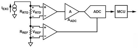
Figure 1: RTD interfacing hardware configuration.
In Figure 1, a single current source (IEXC) excites both the RTD (RRTD) and a precision reference resistor (RREF) by way of a series connection, generating the ADC input voltage (VRTD) and reference voltage (VREF), respectively.
The normalized digital output of the ADC (zero input = 0 and full-scale input = 1) is simply a ratio of the input voltage to the reference voltage multiplied by the gain stage, AADC.


Notice how IEXC cancels out of the above equation. This means that even if the excitation current changes or is imprecise, the ADC result always corresponds directly to the ratio of the RTD resistance to the reference resistance. Choosing a precision, low drift reference resistor means the RTD resistance can be known to a high degree of precision, even with a much less precise current source.
Applying this same principle using a MicroConverter, Figure 2 shows the ADuC706x connected for interfacing with a 4-wire RTD. Note that this is the same overall topology as shown in Figure 1, except that all of the active components (excitation current source, differential input stages for VRTD and VREF, gain stage AADC, the ADC itself, and a microcontroller) are included internally to the ADuC706x chip. Diode protection and 100Ω resistors serve only to protect the ADuC706x from damage in the event of overvoltage conditions at the terminal block.
Also included are other peripherals, such as serial communication ports for the digital communication paths. Notice also that some passive components have been added for R/C filtering of signals and for protection from overvoltage conditions at the terminal block. This represents a complete implementation, requiring only a power supply and any particular peripheral chip needed for the digital interface, such as an RS-232 or RS-485 line driver/receiver.
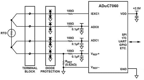
Figure 2: Complete RTD interfacing circuit using the ADuC706x.
Calculating RTD resistance from the ADC results
As introduced in the Hardware Design section,

can be rewritten as:

where:

The scale value is the fixed scaling factor used in the sample code. Taking this a step further, a fixed offset value can be added to the equation, resulting in

where the offset term represents a fixed offset that can be used to compensate for errors. This offset term is discussed further in the Calibration section. In most situations, a value of zero is sufficient for this offset term. Note that a direct equation for RTD resistance is obtained as a function of the ADC result using only a pair of fixed values for scale and offset.
The remainder of this application note considers the most common type of platinum RTD, which has a nominal resistance (R0) of 100Ω at 0°C. When using this application note, assume a reference resistor value of 5.62 kΩ, which provides a good match to such an RTD. With these component values, and using the ADuC706x, an internal gain of 32 is the highest available ADC gain setting that still allows the RTD to cover its fully specified temperature range.
Remember, ADCnorm is limited to the range of 0 to 1, which is what defines the temperature range limitation at higher ADC gains. The gain of 32 corresponds to an ADC0CON value of 0x8415, or a range setting of 37.5 mV unipolar, where:

To correspond to this gain setting, the scale value works out to 175.625, where:

which is the default scale value used in the sample code. The default value for the offset term is zero. These equations assume an excitation current of 200 µA on the IEXC0 pin. This is configured by setting IEXCCON = 0x42.
The equations in this section for RRTD are merely methods of determining, through software, the RTD resistance directly from a given ADC conversion result. To determine the RTD temperature as a function of its resistance requires an understanding of the RTD transfer function.
RTD transfer function
A platinum RTD transfer function is described by two distinct polynomial equations: one for temperatures below 0°C and another for temperatures above 0°C.
The equation for t ≤ 0°C is:

The equation for t ≥ 0°C is:

where for both equations:
t is RTD temperature (°C)
RRTD(t) = RTD resistance as a function of RTD temperature (t)
R0 is the RTD resistance at 0°C (most often 100Ω)
A = 3.9083 × 10⁻³°C–1
B = –5.775 × 10⁻⁷°C–2
C = –4.183 × 10⁻¹²°C–4
Notice that the notation is changed from RRTD to RRTD(t) to reflect that the RTD resistance is a function of its temperature. Figure 3 shows the RTD transfer function (resistance plotted as a function of temperature) along with a linear expansion of the transfer function’s slope at 0°C (for visual comparison).
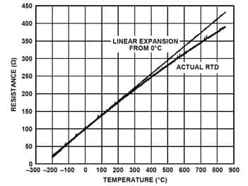
Figure 3: RTD transfer function.
The previous equations define the RTD resistance as a function of its temperature, RRTD(t). However, to implement an RTD sensor interfacing circuit, the RTD temperature must be determined as a function of its resistance, TRTD(r). This may be less straightforward, given the nonlinear transfer function of the RTD. Useful techniques for this task are explored in the following sections.
Linearization techniques
There are many different ways to determine temperature as a function of RTD resistance, given the RTD transfer function. This application note examines three techniques useful in embedded designs. These techniques are particularly well suited to MicroConverter-based designs. Table 1 outlines the strengths and weaknesses of each method. Execution times indicated here represent empirical measurements of an ADuC7060, at a core clock speed of 10.24 MHz, running the C subroutines referenced herein.
| Technique | Advantages | Disadvantages | Summary |
| Direct Mathematical Method | Very accurate. No look-up table required. |
Requires math library (usually>1kB). Slow. | Useful if math library is already used. |
| Single Linear Approximation Method | Very fast (<56µs). Small code space needed. Accurate over narrow temperature bands. No look-up table required. No math library required. | Poor accuracy over wide temperature range. | A good option when limited code space is available and with small temperature span. |
| Piecewise Linear Approximation Method | Fast (<1ms). Designer control of code size and accuracy trade-off. Can be very accurate. No math library required. | Greater code size than single linear approximation method. | Most useful in most situations. |
Table 1: Comparison of linearization methods.
Direct Mathematical Method
In the RTD Transfer Function section, explicit mathematical equations are shown for RTD resistance as a function of its temperature, RRTD(t). Is it possible to just turn those equations around and solve for expressions of the RTD temperature as a function of its resistance, TRTD(r)? This is a fairly straight-forward task for the equation that defines positive temperature behavior because it is merely a quadratic. The solution to the quadratic yields two expressions; to determine which one is correct, simply substitute several known values. The result is the following equation for RTD temperature at temperatures of 0°C or greater:

where:
A = 3.9083 × 10⁻³°C–1
B = –5.775 × 10⁻⁷°C–2
R0 is the RTD resistance at 0°C (most often 100Ω). r is the RTD resistance.
Because this function is solved in real-time, it is beneficial to change it to the following form:

where:
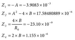
This is advantageous for real-time computation because Z1 through Z4 are constant and absolute, so fewer computations are required. The above equation for TRTD(r) is referred to as the positive function because it relates to temperatures of 0°C and above. Since this is a direct mathematical solution, it is 100 percent accurate within that range. When solving this equation, rounding errors using 32-bit floating-point math in ARM7 C code works out to about +0.0001°C/–0.0005°C. This is close enough to 100 percent accuracy for any practical purposes. When using the ADuC706x with a core clock speed of 10.24 MHz running the sample C routine of RTDmath.c, the execution time of this equation is less than 750 µs.
The previous equation is valid only for temperatures of 0°C and above. The equation for RRTD(t) that defines negative temperature behavior is a fourth-order polynomial (after expanding the third term) and is impractical to solve for a single expression of temperature as a function of resistance. However, making use of computer math tools can assist in finding a close approximation to the inverse transfer function.
Use Mathematica® or a similar software math tool to come up with the following best-fit polynomial expressions for RTD temperature at temperatures of 0°C or less:
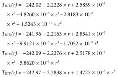
These four equations are referred to as the negative functions because each is valid only for temperatures of 0°C and below. The top (fifth-order) equation is the most accurate, but takes the longest time to compute, while the bottom (second-order) equation is the least accurate, but is the fastest to compute. Some characteristics of these negative functions are given in Table 2, and a plot of the error of each as a function of temperature is shown in Figure 4 along with (for visual reference) the error of the positive function extended into the negative temperature space.
Notice in Figure 4 that at near-zero negative temperatures, there is actually less error in the positive function than in the second-, third-, or fourth-order negative functions. The sample code RTDmath.c takes advantage of this behavior by using the positive function even at slightly negative temperatures. The actual threshold to determine if the positive or negative function should be used differs depending on which negative function (second-, third-, fourth-, or fifth-order) is used, and is represented in the Threshold column of Table 2. Above this threshold value, the positive function yields lower errors; below this threshold value, the negative function yields lower errors. The Equation Accuracy column in Table 2 represents errors only for temperatures below the corresponding threshold value.
| Equation Size | Maximum Execution Time¹ | Equation Accuracy¹ | Threshold |
| Fifth Order | 2.16 ms | +0.0001°C/-0.00005°C | 0°C/100Ω |
| Fourth Order | 1.61 ms | +0.0022°C/-0.001°C | -8.75°C/+96.6Ω |
| Third Order | 1.13 ms | +0.0053°C/-0.0085°C | -12.5°C/+95.1Ω |
| Second Order | 800 µs | +0.075°C/-0.17°C | -70.5°C/+72.1Ω |
¹Execution time and equation accuracy were measured empirically on an ADuC706x, at a core clock speed of 10.24 MHz, running the sample C routine of RTDmath.c.
Table 2: Characteristics of best-fit polynomial equations (negative functions).
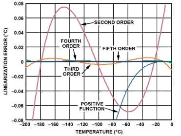
Figure 4: Error plot of best-fit polynomial equations (negative functions).
One drawback of the direct mathematical technique for linearization is that it requires floating-point power and square root functions such as those found in the math library of the IAR compiler from IAR Systems. These floating-point math functions alone typically add more than 1kB to the code size. Similar or better accuracy can be achieved with smaller overall code size using the piecewise linear approximation method described in the Piecewise Linear Approximation Method section. However, if the math library functions are required for other operations in the program, the direct mathematical technique may be the best solution because those library functions are already available.
Single Linear Approximation Method
In Figure 3, notice that over smaller temperature spans the RTD transfer function resembles a straight line. If the required measurement temperature range spans only a portion of the full RTD measurement band, the RTD signal might not need to be linearized at all. In such cases, a best-fit linear approximation to the transfer function over the desired measurement temperature range can often yield sufficient precision. For example, over the industrial temperature range of –40°C to +85°C, a best-fit linear approximation is accurate to ±0.3°C.
In general, a linear equation for temperature as a function of RTD resistance (r) is of the form:

where A and B are constants.
Note that these are not the same A and B as described in the RTD Transfer Function section. Choosing optimum values for A and B to minimize the error band involves some math not explored here. There is, however, a very simple software tool that accompanies this application note, that can automatically find optimum values of A and B to fit your specific temperature range. This tool is examined in this application note, but first it must be determined whether a single linear approximation is suitable for the specific design requirement.
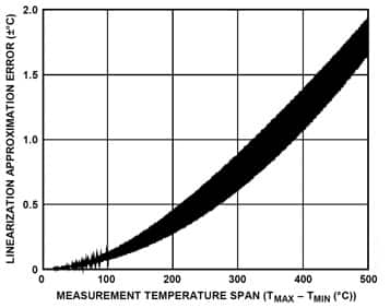
Figure 5: Single linear approximation error vs. measurement temperature span.
Figure 5 offers a view of the total approximation error that results for measurement temperature spans of up to 500°C. For more than 500°C spans, the approximation error continues to degrade with increasing temperature spans. The imprecise nature of the Figure 5 plot (that is, the broad width of the data trace) is due to the fact that even for the same span of temperature, the error is different for different absolute temperature bands. For example, the temperature ranges of –200°C to 0°C and +600°C to +800°C do not have the same precision even though they both span exactly 200°C.
Figure 5 provides a rough idea of error to help gauge whether single linear approximation should be considered as an option. If it is determined that it might be an option, the RTD coefficient generator tool (described in the RTD Coefficient Generator Tool section) can help determine the actual approximation error for a specific temperature range, and can generate source code optimized for that temperature range.
Piecewise linear approximation method
Taking linear approximation one step further, one can conceptualize any number of linear segments strung together to better approximate the nonlinear RTD transfer function. Generating this series of linear segments so that each segment’s endpoints meet those of neighboring segments results in what can be viewed as a number of points connected by straight lines. These points (or coefficients) can be calculated once to best match the nonlinear transfer function of the RTD and then stored permanently in ROM or flash memory. From this table of coefficients, the MCU can perform simple linear interpolation to determine temperature based on measured RTD resistance.
To understand how this is implemented in practice, first assume the table of coefficients already exists. Each coefficient in the table is simply a point on the transfer function, represented by a resistance and a temperature. Thus, the table takes the form:

Given this table, the real-time task of the MCU (in determining temperature at a given resistance, r) is to first determine which two coefficients are closest to the point in question (call these {rm,Tm} and {rn,Tn}), and then to linearly interpolate between those two points to solve for temperature. The actual linear interpolation formula for that range (that is, valid only for values of r between rm and rn) then takes the form:

Note that each coefficient in the above lookup table consists of two numbers, one for resistance and one for temperature (essentially x and y values in the transfer function). Thus, for N linear segments (that is, N + 1 coefficients), a total of 2N + 2 values must be stored in memory. To reduce the size of the lookup table, consider a table consisting of N segments, each spanning an equal breadth of resistance. Such a table can be stored as a set of temperature points only as follows:
{T0; T1; T2; ... tN}
since, for a given coefficient {rn,Tn}, the value of rn can be calculated by:

where:
r0 and rSEG are fixed values, stored in ROM along with the table of coefficients.
r0 is the resistance at coefficient zero {r0,T0}.
rSEG is the fixed span of resistance that separates adjacent coefficients.
The linear interpolation formula for a given segment then becomes

where i indicates which segment (that is, which pair of coefficients) is being used, and is calculated using the value of r as follows:

Again, the above expression for TSEG(r) is nothing more than a linear interpolation between the two coefficients, Ti and Ti + 1. To implement this in practice, the MCU must first solve for i (per the last equation,) so that the coefficients Ti and Ti + 1 are the two closest to the input value for r. Then, with i solved, the MCU can simply solve the TSEG(r) equation to determine the temperature at the given input resistance.
The overall error generated by this piecewise linear approximation technique depends on the number of segments (or number of coefficients, or the size of lookup table), and the overall span of temperature.
Figure 6 shows the linear approximation error for a measurement temperature range of –200°C to +850°C plotted as a function of lookup table size (using optimized coefficients generated by the RTD coefficient generator tool). Note that if the measurement temperature range is reduced, a better error results given the same size lookup table, or the same error results given a smaller look-up table.
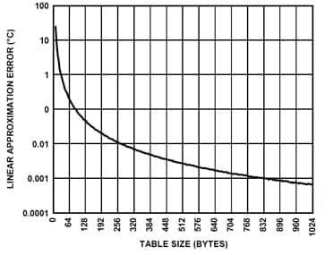
Figure 6: Piecewise linear approximation error vs. look-up table size (-200°C to +850°C range).
RTD Coefficient Generator Tool
The most difficult part of implementing a piecewise linearization function is generating the lookup table. However, the RTD coefficient generator tool that accompanies this application note (coefRTD.exe) does this automatically for platinum RTDs. This simple DOSexecutable assists with ARM7-based RTD interface designs using piecewise linear or single linear approximation methods. It performs the following tasks:
- Generates optimized lookup table coefficients for a given temperature range and look-up table size.
- Indicates resulting error band and lookup table size.
- Generates complete RTD linearization functions (including the lookup table) in ARM7 C source code.
- Generates a table of error values as a function of temperature resulting from the given lookup table.
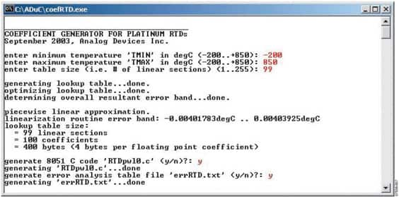
Figure 7: Coefficient generator session example with piecewise linear approximation (user input in red).
Figure 7 shows a sample session with user input. Note that the program requires the user to input only three parameters (TMIN, TMAX, and NSEG). The program can generate the file RTDpwl0.c, which is a complete C source file (a customized, user specific lookup table) that can be included as is in a project where the T_rtd() function is available to be called directly from functions in other source files. Alternatively, any portion(s) of RTDpwl0.c can be copied and pasted directly into other source file(s).
The coefficient generator can also output an error analysis file (errorRTD.txt), which is a tab-delimited text file that can be imported into Microsoft® Excel or any other spreadsheet program to examine the errors generated by the linear approximation routine.
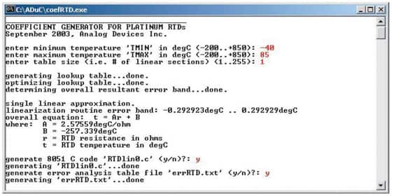
Figure 8: Coefficient generator session example with single linear approximation (user input in red).
The coefficient generator program generates linearization functions not only for piecewise linear approximation, but also for single linear approximation. To do this, enter 1 for the table size to indicate only a single linear segment.
The program recognizes this and outputs results pertaining to the single linear approximation method instead of the piece-wise linear approximation method, as shown in Figure 8.
Calibration
The ADuC706x has a built-in function to calibrate the ADC for endpoint errors (offset and gain error) as documented in the product data sheet. However, if the entire signal chain, including the RTD itself, is taken into account during calibration, one can end up with a lower overall error, and in such a case, the built-in ADC calibration provides no added benefit. This application note examines the overall calibration first, and then points out some instances where the built-in ADC calibration may still be useful.
Up to this point, the assumption has been that the RTD itself is perfect. However, real RTDs are not perfect. Just like anything else in the real world, they have errors associated with them as specified by the RTD manufacturer’s data sheet. Fortunately, many of these errors can easily be calibrated out in software. The calibration function discussed in this application note works as either a single-point or a two-point calibration. This function can be used in conjunction with any of the linearization techniques.
To understand how a single-point calibration works in principle, refer to where RRTD(t) is discussed in the RTD Transfer Function section and note that it is largely defined by the value R0, which is the resistance of the RTD at 0°C. For the most common RTDs, R0 is nominally 100Ω. However, this R0 value is the most significant source of error in an RTD sensor because it can vary significantly from one device to another. In addition, because the R0 value is simply multiplied by the rest of the transfer function in the expressions for RRTD(t), errors due to R0 tolerance are purely multiplicative, and so can be corrected by adjusting the scale multiplier in the following expression (as given previously) for RRTD as a function of normalized ADC conversion result:

Specifically, if the RTD can be brought to a very precise known temperature and an ADC conversion performed, then the corrected scale value can be calculated as:

where ADCcal is the actual normalized result of the analog-to-digital conversion and Rcal is the ideal (expected) resistance value at that RTD temperature. Rcal can be calculated manually using the equations for RRTD(t). By this method (called single-point calibration), a corrected scale value is obtained, compensating for the RTD R0 tolerance and also, simultaneously, for the reference resistor’s initial tolerance. To take this a step further, one can employ a two-point calibration, which compensates not only for these scaling errors, but also for any offset error that may exist. Doing so requires adjusting not only the scale value, but the offset value as well.
Assume that a single-point calibration has already been performed, and the RTD can now be brought to a second very precise known temperature, and another ADC conversion is performed. The equation for the scale value (that is, the slope of the RRTD vs. ADCnorm function) is then:

where:
Rprecal and ADCprecal are the resistance and ADC conversion result, respectively, at the previous calibration point.
Rprecal and ADCprecal are the same for the current calibration point.
Note that this is a way of determining the slope of the RRTD vs. ADCnorm transfer function using two points on that line. One has only to take care of the offset value, which, because the scale value is now known, can be determined using a single point. The following expression for the offset value comes by solving for the offset of the above RRTD expression and then replacing RRTD and ADCnorm with Rprecal and ADCprecal, respectively.

Note that if Rprecal and ADCprecal are both zero (representing no prior calibration point), then the expression for the scale value becomes the same as for a single-point calibration, and the expression for the offset value becomes zero, just as if this were a single-point calibration. Therefore, the same function (Cal() in the sample code) can be used to perform either a single-point or a two-point calibration.
If using the sample code as is, follow these steps to perform a 2-point calibration:
- Choose two temperatures for calibration, making sure that the temperature points are sufficiently separated (ideally at least one quarter of the total measurement span) to avoid errors accumulating near the extremes of the measurement temperature range.
- Bring the RTD to the first temperature point, wait for the displayed result to settle to the new value, and then press any key on the terminal (or terminal emulator) to display the user I/O menu.
- Follow the menu prompts to calibrate to a known temperature, and then enter the temperature when prompted.
- Repeat Step 2 and Step 3 for the second temperature point.
Although there are many benefits to calibration, there are just as many system considerations that make it impractical for certain applications. If a calibration cannot be performed as described in Step 1 through Step 4, consider performing a system ADC calibration instead, as described in the ADuC706x data sheet. To do so, replace the RTD with a short resistance (0Ω) and trigger a system zero-scale calibration. Then, replace the RTD with a high precision 719.36Ω resistance and trigger a full-scale calibration. This compensates for internal ADC errors and for initial tolerance of the RREF resistor, but does not account for any errors of the RTD itself.
Note that an added benefit of the ADuC706x (and all other MicroConverter products) is that it includes nonvolatile Flash memory on-chip, which can be used to store the calibrated scale and offset values. This way, the chip can restore the calibrated values each time the system powers up, rather than requiring a calibration each time the system is powered up.
Error analysis
There are many contributing error sources to data acquisition designs, such as ADC linearity, input amplifier noise, resistor Johnson noise, amplifier temperature drift, and resistor temperature drift. Determining which ones are dominant for a given design can be a daunting task. Fortunately, the ADuC706x integrates all the active stages into a single fully factory-specified device, making error analysis a much simpler task, but one that still requires insight in designs that involve a nonlinear sensor element. This application note explores the few error components that are most significant for the specific hardware and software configurations discussed thus far.
If the system is not calibrated to a specific RTD (using the single-point or two-point calibration), the RTD itself is almost certainly the most significant source of absolute error. This error, which should be well quantified in the RTD manufacturer’s data sheet, depends on the specific model of RTD chosen. This application note concentrates on error sources other than the RTD itself.
Noise
One type of error to examine is noise. There are three main noise sources to consider in this design: resistor Johnson noise, amplifier/ADC input voltage noise, and amplifier/ADC input current noise. These add together as a root-sum-of-square, and so the lesser contributing sources are negligible when one noise source is even slightly greater than another source. In this specific case, that dominant noise source happens to be amplifier/ADC input voltage noise. Specifically, at the gain setting discussed, the ADuC706x input voltage noise specification is 0.25 µV rms, or about 1.65 µV p-p.
Translating this input voltage noise into the resulting output temperature noise may not be intuitively obvious and, because of the nonlinear resistance-to-temperature transfer function, results in a temperature noise that varies as a function of RTD temperature. The result is shown in Figure 9.
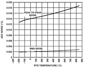
Figure 9: ADC noise vs. RTD temperature.
Notice that even at the highest RTD temperatures (that is, the worst noise), peak-to-peak noise is always below 0.013°C; it is even better at lower measurement temperatures. Keep in mind that this variation of noise as a function of RTD temperature is not a function of the ADC itself but rather, is a direct result of the nonlinear TRTD(r) transfer function implemented in the digital domain.
Temperature drift
Another source of error to consider is temperature drift; specifically, ADC offset and gain temperature drift and reference resistor temperature drift. This is the change in dc errors (offset and gain errors) as a function of changing temperature of the ADC chip or reference resistor. This relates to ambient temperature of the RTD conditioning circuitry rather than to the actual measured RTD temperature. Briefly, these two distinct temperatures are referred to here as ambient temperature and RTD temperature, respectively. In addition, the value of temperature drift (that is, sensitivity to ambient temperature) changes as a function of RTD temperature due to the nonlinear TRTD(r) transfer function. The result shown in Figure 10 requires some explanation.
The x-axis of Figure 10 is the RTD temperature. The y-axis is the temperature drift in °C change in measurement error per °C change in ambient temperature. For example, if the RTD temperature is fixed at 100°C, the VREF drift (with a 5 ppm/°C reference resistor) is approximately ±0.01°C/°C. Therefore, if the ambient temperature changes by, for example, 50°C, the measurement temperature reading may change by as much as ±0.5°C (neglecting other contributors to temperature drift).
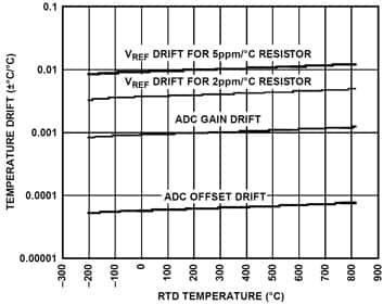
Figure 10: Temperature drift vs. RTD temperature.
It is evident that in industrial environments with ambient temperature ranges often spanning -40°C to +85°C or more, temperature drift can be quite a significant source of error. It is straightforward to use the on-chip temperature sensor of the ADuC706x to measure chip temperature (which tracks ambient temperature closely) and then use this measured chip/ambient temperature to compensate for temperature drift errors.
This requires an additional temperature cycling step during manufacturing, specifically bringing the ambient temperature to two fixed values and taking zero-scale and full-scale ADC readings at each of these ambient temperatures. However, software can be used to compensate for temperature drift errors within the limits of temperature sensor accuracy and temperature gradients between the reference resistor and the ADuC706x. This application note does not explore such temperature drift compensation techniques any further; however, note that the on-chip resources exist to make this option possible with nothing more than software changes.
RTD self-heating
RTD self-heating is another source of error to consider. Simply put, placing a current through the RTD causes it to dissipate power, which raises the temperature of the RTD. Fortunately, because the RTD is being excited with only 200 µA, the total power dissipated by the RTD is never more than 8 µW for a 100 Ω R0. The amount of self-heating caused by this small power dissipation varies, depending on the specific model of RTD used, but typically the resulting self-heating is negligible.
Other error sources
Other sources of error are mostly negligible. DC endpoint errors (offset and gain errors) can be fully corrected using the calibration techniques discussed in the Calibration section. Resistor Johnson noise is well below the input voltage noise of the ADC. The only other error source worthy of consideration is ADC INL (integral nonlinearity or relative accuracy). The ADuC706x data sheet specification for typical INL is 15 ppm of full scale, which results in output-referred INL error about twice the value of the peak-to-peak output noise shown in Figure 9.
Software and source code
All of the software and source code referenced in this section is included in a zip file. This file is available at www.analog.com/MicroConverter. The contents of the zip file are as follows:
- coefRTD.exe. The coefficient generator tool executable.
- coefRTD.cpp. Source code for the coefficient generator tool.
- RTDdirect.c. Linearization subroutines using the direct mathematical linearization method.
- RTDpwl.c. Linearization subroutines using the piecewise linear approximation method. A customized version of this code can be generated using the coefRTD.exe program.
- RTDlin.c. Linearization subroutines using the single linear approximation method. A customized version of this code can be generated using the coefRTD.exe program.
- RTDLinearMain.c. An example of a complete RTD inter-face program for the ADuC706x. This makes use of any of the three linearization functions.
- RTDLinearMain.hex. A complete compiled version of RTDLinearMain.c and RTDpwl.c. This is ready to download and run on an ADuC706x.
- Calibrate.c. Example code providing subroutines for calibrating an external RTD.
- ReadMe.txt. Text file providing revision information and describing the function of each file.
- A complete project using the above source code must include both a main program (RTDLinearMain.c, Calibrate.c, or a from-scratch program) and a linearization subroutines file (RTDmath.c, RTDpwl0.c, RTDlin0.c, or a customized source file generated by the coefRTD. exe tool). Many details are provided in the comments of the various C source files.
- An IAR example project.

免责声明:各个作者和/或论坛参与者在本网站发表的观点、看法和意见不代表 DigiKey 的观点、看法和意见,也不代表 DigiKey 官方政策。


